
Everything you need to know about the VLOOKUP() function in Excel
Whether you're analyzing financial data, preparing a sales report, or managing a list of customer information, it's often essential to combine information from different sources. This is where the VLOOKUP() function in Excel comes in handy. This feature allows you to look up values in a specific column and retrieve matching data from another column, similar to a dictionary or reference book. In this article we will delve deeper into how the VLOOKUP() function works and how to resolve possible error messages.
The VLOOKUP function
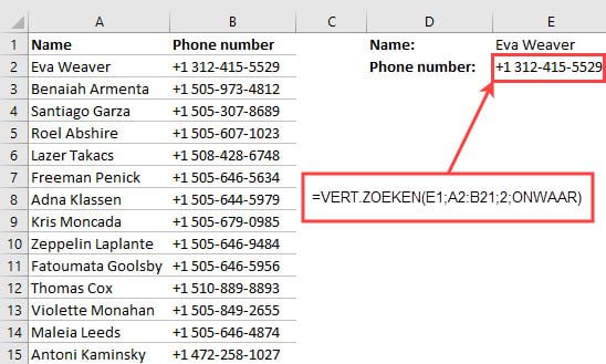
The VLOOKUP() function is one of the most powerful tools in Excel for combining data from multiple tables. The function searches for a specified value in the first column of a specified range (often a different table) and returns the corresponding value from another column in that same range. The syntax of the VLOOKUP function is structured as follows:
VLOOKUP(search_value, table_array, column_index_number, [approach])VLOOKUP arguments
| search value | The search value can consist of a value or a reference to a cell. The value you want to look up must be in the first row of the cell range. |
| table matrix | The cell range in which VLOOKUP searches for the search value and the search value. The first column in the cell range must contain the search value. The cell range must also contain the return value you want to find. |
| columnindex_number | Enter the column number of the column from which the value should be returned. The leftmost column of the table matrix is column number 1. |
| approach (optional) |
|
Possible error messages and solutions
VLOOKUP returns a #N/B error
The error message #N/B means that Excel cannot find the search value in the specified table matrix. Verify that the search value is spelled correctly and matches the values in the first column of the table array.
One of the main limitations of Excel VLOOKUP is that it cannot look to the left. Therefore, a lookup column should always be the leftmost column in the table array. In practice we often forget this and end up with #N/A errors.
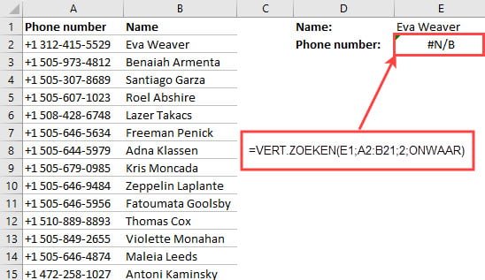
Suppose you have a list of names and phone numbers in a table array. If you try to look up a person's phone number using the VLOOKUP() function, but the name does not appear in the table array, the error message #N/B is returned.
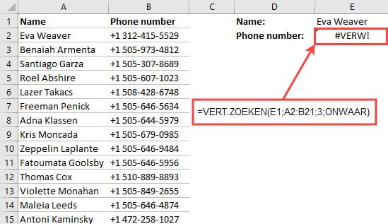
VLOOKUP returns the error #REF!
This error occurs when the specified column_index is outside the range of the table array. This happens if the specified number does not match the number of columns in the table array.
VLOOKUP returns the error #ARG
This error occurs if there is an error in the function's arguments. This can happen if the syntax of the function is wrong.
Limitations of the VLOOKUP() function
Although the VLOOKUP() function is a powerful tool for finding and combining data in Excel, it also has some limitations. Here are some of the main limitations of the VLOOKUP() function:
Search in one direction
The VLOOKUP() function always searches for values in the first column of the specified table array and returns values to the right of this column in the same row. This means that the function only searches in one direction (vertical).
If it is not possible to restructure your data so that the lookup column is the leftmost column, you can use the functions INDEX and MATCH together as an alternative to VLOOKUP
Exact match
By default, the VLOOKUP() function searches for exact matches between the search value and the values in the first column of the table array. If there is not an exact match, the function displays an error message (#N/B). Although you can use the [approximate] argument to allow an approximate match, this can sometimes lead to unexpected results.
One result per search value
The VLOOKUP() function returns only one result per search value, even if there are multiple matching values in the table array. If there are multiple matching values, the function will return the first matching value and ignore the rest.
Search in the leftmost column
When using the VLOOKUP() function, make sure that the search value is in the leftmost column of the table array. Otherwise the function will not find the search value.
The VLOOKUP() function searches for a value in the left column of the specified table array and returns values from the same row in another column of that array. This means that the function searches along the vertical dimension of the table array, with the search value in the left column and the return value in another column in the same row.
Sensitivity to error
The VLOOKUP() function can be prone to human error, such as misspellings when entering search values or incorrectly setting the [approach] argument. This may lead to unexpected results or error messages.
Efficiency with large data sets
When searching large data sets, the VLOOKUP() function may cause some delays and affect the performance of your spreadsheet. In such cases, using other functions such as INDEX and MATCH can sometimes be more efficient.
In Excel versions up to and including Excel 2010, the maximum number of rows in which you can use the VLOOKUP function is 1,048,576 rows. This corresponds to the maximum number of rows in a worksheet in these versions of Excel.
In newer versions of Excel, such as Excel 2013, Excel 2016, Excel 2019, and Excel 365, this maximum number of rows has remained the same: 1,048,576 rows.
This means that you can use the VLOOKUP function to look up data in a table array with up to 1,048,576 rows. If you have data that exceeds this limit, you may need to consider other approaches, such as splitting the data into multiple tables or using other Excel functions.
If the above explanation doesn't work out for you, you can download a sample file below.
terbinafine antifungal summary
terbinafine antifungal summary
vidalista side effects
vidalista side effects
voriconazole for uti
voriconazole for uti
cialis indian pharmacy
cialis indian pharmacy
prevacid 30 mg generic
prevacid 30 mg generic
hello world
hello world